


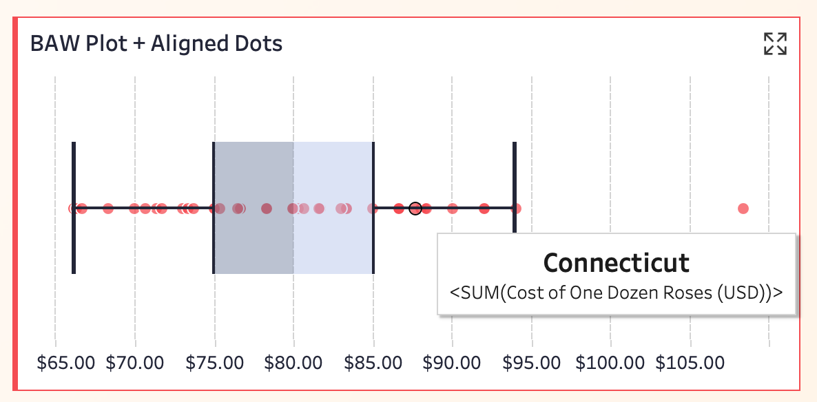
Alternatives to Box Plots: N Ways to Visualize Data Distribution in Tableau
Alternatives to Box Plots: N Ways to Visualize Data Distribution in Tableau
In daily analysis, distribution visualization is one of the most effective ways to reveal data details and characteristics. For example, many people use box plots to display metrics like the median, quartiles, and outliers of a dataset. But can a box plot alone truly capture all the nuances of data distribution?
Inspired by this question and the “Data Visualization Catalogue,” data enthusiast Kevin Wee created a Viz exploring “Box Plots and Their Better Alternatives” based on a dataset of rose prices across U.S. states. He analyzed the strengths and ideal use cases for each alternative.
Today, let’s dive into this Viz and discover how to choose the most suitable chart for your data distribution needs!
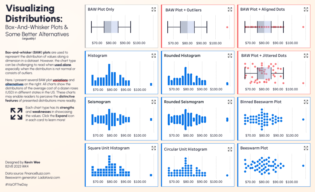
01 Standard Box Plot
As one of the earliest distribution visualizations many encounter, a box plot uses a “box” and “whiskers” to quickly summarize data distribution: where the data is concentrated and its overall range.
As shown below, this is a classic box plot:
The ends of the box represent the upper and lower quartiles.
The middle line is the median, meaning the box covers the median and the interquartile range (IQR).
The “whiskers” extend to the lower and upper bounds of the data, typically 1.5 times the IQR. Extreme values (outliers) are often omitted.
From the data, the box spans $74.96 to $85.00, indicating that over half of the prices fall in this range. The median line ($79.98) represents the “waistline” of the distribution. The whiskers show the spread beyond the quartiles, providing an overview of price fluctuations.
In other words, rose prices in most U.S. states are concentrated between $75 and $85, with no extreme outliers. The distribution is relatively symmetrical.
However, Kevin does not recommend relying solely on box plots for distribution analysis and suggests pairing them with other distribution charts.
Pros: Ideal for comparing multiple datasets or quickly understanding the spread and central tendency of a single dataset.
Limitations: Struggles to reveal detailed distribution patterns, especially for skewed data or datasets with many outliers. Different tools may define whiskers differently, affecting interpretation.
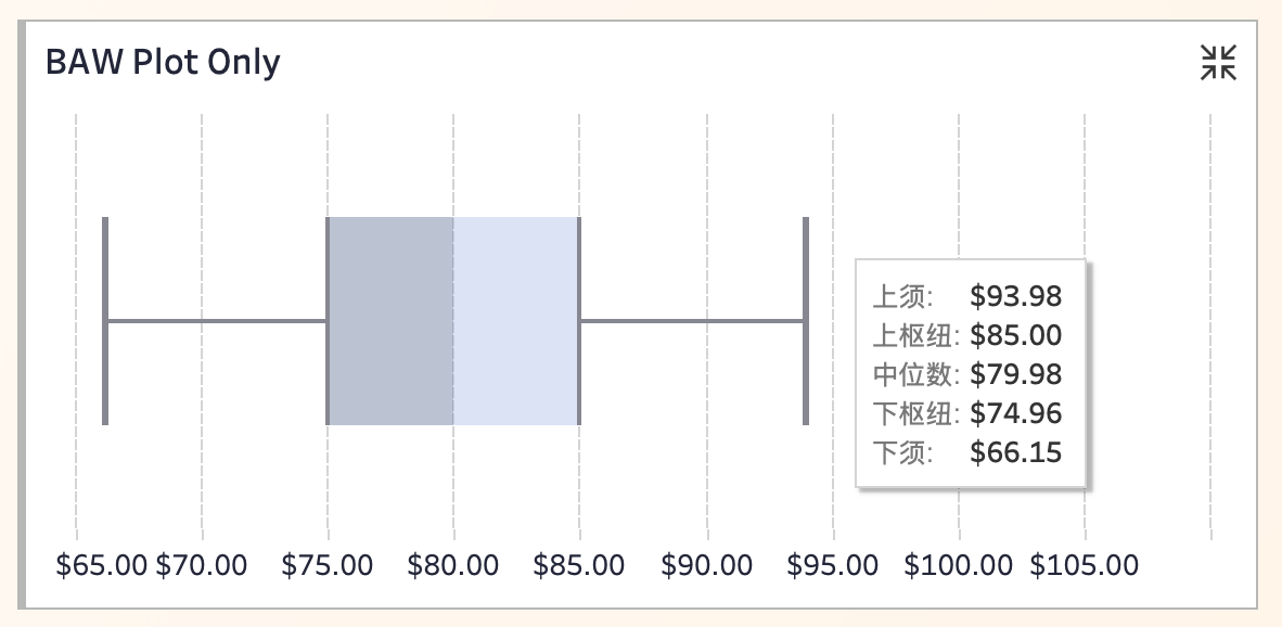
02 Box Plot + Outliers
Unlike the standard box plot, this version explicitly marks outliers (data points beyond the normal range) with red dots, making extreme values immediately visible.
From the data, most states’ rose prices fall between $75 and $85. The red outlier on the right represents Hawaii, where prices are significantly higher than the norm.
Pros: Easily identifies the main distribution range and highlights outliers. For example, Hawaii’s price would be hidden in a standard box plot but is clearly visible here.
Limitations: Still lacks sensitivity to internal distribution details, such as local density or clustered ranges.
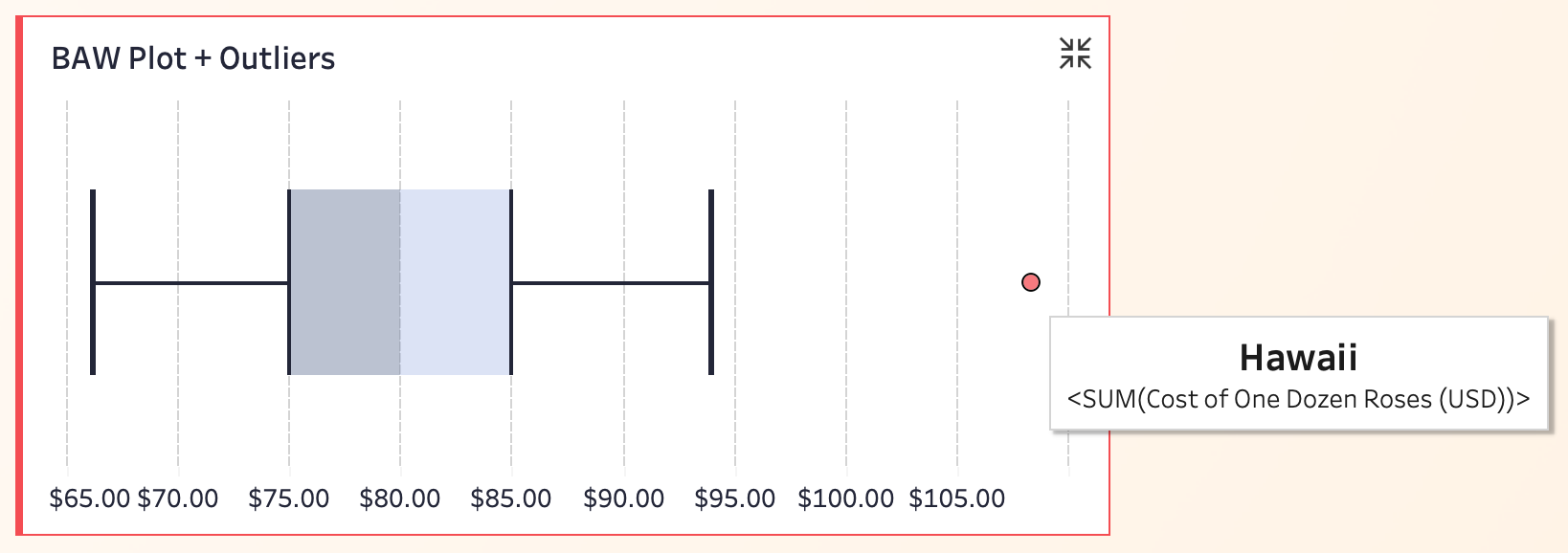
03 Box Plot + Aligned Points
This approach plots each state’s price as a dot aligned along the median line, preserving both distribution trends and individual values.
For example, Connecticut’s price is around $90.00, near the upper whisker—relatively high but not an outlier.
Pros: Combines the benefits of box plots with granular data inspection, serving both macro and micro analysis needs.
Limitations:
Dots may overlap excessively with large datasets.
Some points may be obscured by the box in dense regions.
Whisker definitions can still vary.
For implementation tips, see: Example! Tableau Tip: Using Violin Plots to Show Data Density in Box Plots.
04 Histogram
Histograms offer a more intuitive and detailed way to visualize distributions. While box plots emphasize quartiles and outliers, histograms show the count of observations in each bin, making the distribution structure clear.
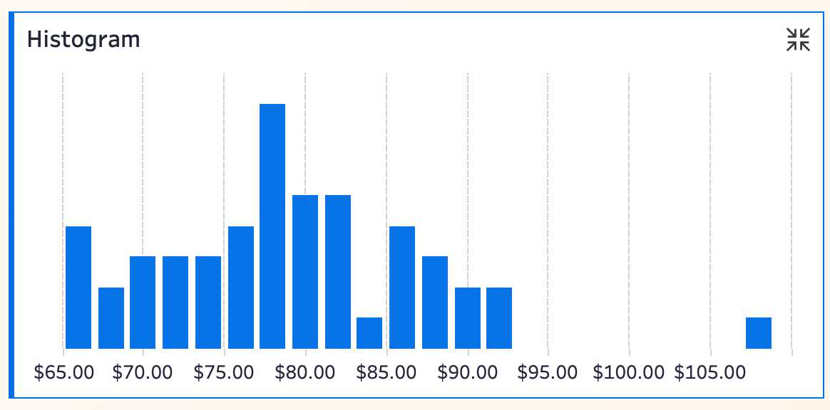
For example, the $78.00–$79.99 bin contains 8 states—the densest price range. Unlike box plots, histograms quantify exactly how many states fall into each price range. The single outlier above $105 (Hawaii) is also visible.
Pros: Clearly reveals “peaks” and “valleys” in the data, ideal for large or unevenly distributed datasets. The “bin” concept is intuitive and easy to explain.
Limitations: Distribution appearance depends on bin width—too wide hides details; too narrow looks cluttered. Tableau’s auto-binning may require manual adjustment.
05 Rounded Histogram
This is a stylistic upgrade to the standard histogram, replacing rectangular bars with rounded ones.
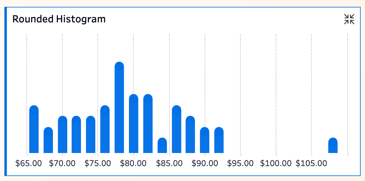
While the data insights remain the same, the rounded design is visually softer. The aesthetic improvement may not justify the extra effort unless presentation polish is a priority.
06 Box Plot + Jittered Points
This variant randomly disperses points vertically to prevent overlap, making density patterns visible.
Most prices cluster between $75 and $85, with Hawaii’s outlier still prominent.
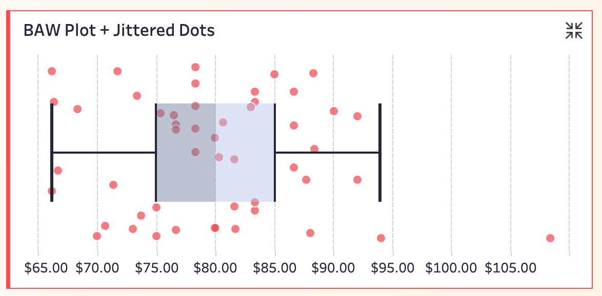
Pros: Solves overlap issues, enriches detail, and highlights outliers.
Limitations: The jittered Y-axis is meaningless and may confuse beginners. Overplotting can still occur in dense regions.
For implementation, see: Example! Tableau Tip: Using Jitter Plots to Show Box Plot Distributions.
07 Seismogram
Think of a seismogram as a mirrored histogram. It symmetrically unfolds the distribution along a central axis, resembling seismic or sound waves. This enhances the sense of distribution layers, making peaks and valleys more obvious.
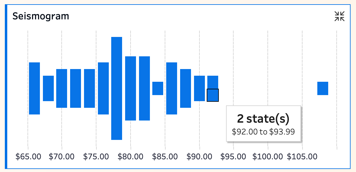
For example, the peak around $80 is the dominant price range, while the $85–$87 “valley” is sparse. The $105+ outlier stands alone.
Pros: Better than histograms at showing overall trends and local variations, especially for irregular distributions. Kevin rates it highly for balancing macro and micro insights.
Limitations: Still sensitive to bin width. The mirrored layout may require acclimation.
08 Rounded Seismogram
A stylistic upgrade to the seismogram with rounded bars for a softer, modern look.
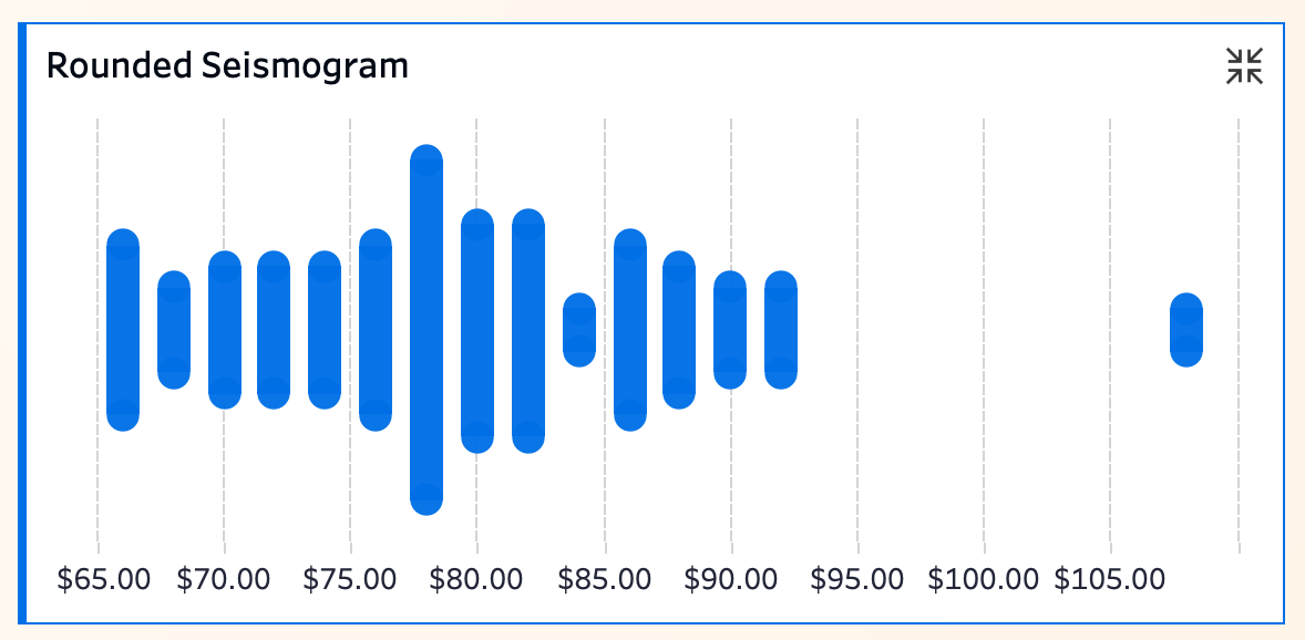
Pros: Retains all seismogram advantages while improving aesthetics.
Limitations: No substantive informational gain. Design complexity increases with large datasets.
09 Binned Beeswarm Plot
This hybrid uses circles to represent observations, stacked vertically within each price bin. The taller the stack, the denser the data in that bin.
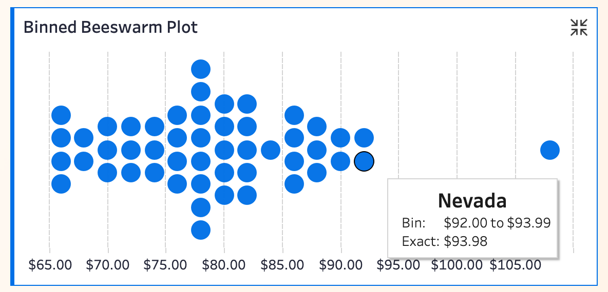
Pros: For small datasets, it’s easier to count exact values per bin than estimate bar heights. The circular layout is visually friendly.
Limitations: Readability depends on bin width. Overplotting worsens with large datasets.
10 Square Unit Histogram
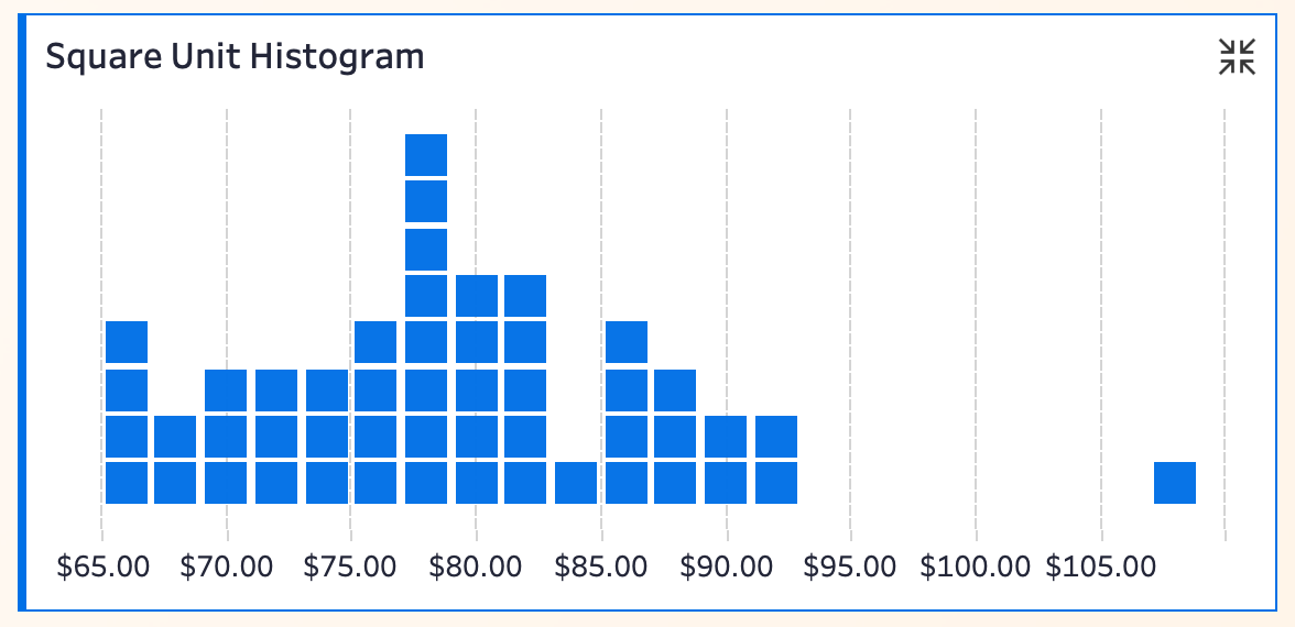
Here, each square represents one observation, replacing traditional bars. This lets users count exact values per bin.
Pros: Great for small datasets where granularity matters.
**Limitations”: Gridding can create visual noise. Poor binning obscures patterns. Scalability is limited.
Kevin gives it 3/5 stars, recommending it for small datasets where “showing every point” is key.
11 Circular Unit Histogram
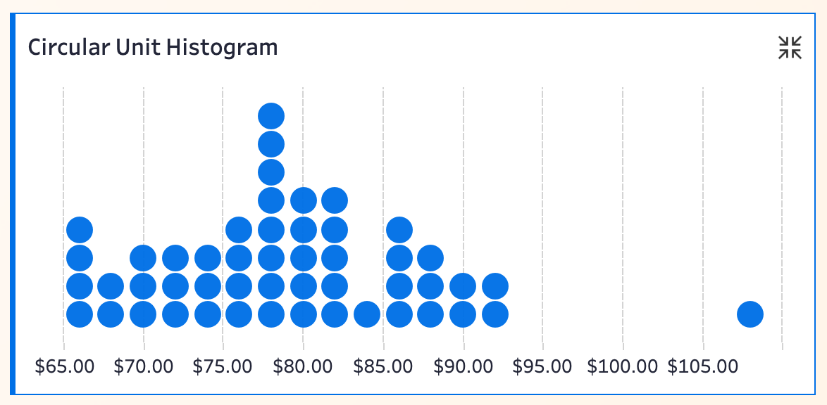
Similar to the square version but uses circles for a softer look.
**Pros”: Combines granularity with visual appeal, ideal for small datasets or non-technical audiences.
**Limitations”: Still bin-width-dependent. Overplotting risks remain.
Kevin rates it 4/5 for balancing detail and aesthetics.
12 Beeswarm Plot

The beeswarm plot positions each dot at its exact value on the X-axis, with vertical jitter to prevent overlap.
**Pros”: Maximizes detail and individual readability, perfect for small datasets or presentations emphasizing each data point.
**Limitations”: Hard to implement natively in Tableau—requires extensions or scripts. Overplotting occurs with large datasets.
Kevin gives it 3/5 due to implementation complexity.
For how-to, see: Example! Tableau Tip: Using Extensions to Create Beeswarm Plots.
Best Practices for Data Distribution Visualization
Choose charts based on data characteristics, analysis goals, and audience expertise:
Box plots: Good for overviews and comparisons, but pair with other charts.
Histograms/seismograms/unit charts: Reveal distribution details; ideal for exploration.
Beeswarm/jittered plots: Show individual points; best for small datasets or outlier analysis.